Contact Info

Location Engineering Building | room 332
Phone 435-797-1494
Contact Christian Bolander
Email christian.bolander@usu.edu

Hours

Mon–Thu	10am – 5pm
Fri	10am – 4pm

Drop-Ins Welcome!

Closed weekends and university holidays.

EMRC Trigonometry Review

Angles

Trigonometry is the study of the relationships between the angles and the lengths of the sides of triangles. An angle is the amount of rotation from an initial ray or line to a terminal ray or line. Figure 1 shows an angle of 45 degrees, where one degree is 1/360 of a full circular rotation. Therefore, a circular rotation contains 360 degrees, written as 360°.

$Representation of an angle in Cartesian coordinates$

Figure 1. Representation of an angle in Cartesian coordinates

In a traditional Cartesian coordinate system (as in Fig. 1), positive angles are measured counterclockwise from the x-axis and negative angles are measured clockwise from the x-axis. Thus, depending on the direction of rotation, the angle between an initial and terminal ray or line can be expressed as a positive or negative number. These angles are called coterminal, a definition that can be used to describe any angles that share the terimal side. Since a circular rotation contains 360°, an infinite number of coterminal angles can be generated by adding 360° to any angle

The quadrant in which an angle is located is also important. Quadrants in a Cartesian coordinate system are defined using the quadrantal angles of 0°, 90°, 180°, 270°, and 360°. The quadrantal angles are measured between the x-axis and the remaining coordinate axes in a Cartesian coordinate system. The first quadrant is between 0° and 90°, the second quadrant is between 90° and 180° and so forth. An angle within each quadrant is shown in Fig. 2.

While the unit of degrees is helpful for the purposes of visualization of rotations, measuring angles in terms of radians is essential for most trigonometric calculations. A radian is defined as the measure of a central angle of a circle that intercepts an arc equal in length to the radius of the circle (see Fig. 3). Based

$Quadrants in a Cartesian coordinate system$

Figure 2. Quadrants in a Cartesian coordinate system.

on the relationship between the circumference of a circle and the degrees in a circular rotation, angles in degrees can be converted to radians through the factor

(1)

θ_{rad} = θ° \frac{2 π}{360°} = θ° \frac{π}{180°}

Question 1. To maintain equilibrium, an aircraft control system with a rotating tail indicates that 382° of rotation is required. With rotation limits on the tail of ±180°, what rotation angle will be equivalent to that given by the control system?

$Definition of a radian$

Figure 3. Definition of a radian.

Right Triangles

A triangle with an interior angle of 90° is called a right triangle. Properties associated with right triangles are extremely important in engineering and will show up consistently throughout your course work. Using a right triangle, we can define the trigonometric functions, which will be discussed next. In relation to an interior, non-right angle θ, the adjacent side is the side closest to the angle that is not directly opposite to the right angle. The side directly opposite to the right angle is called the hypotenuse, and the side across from the angle is called the opposite side.

The first trigonometric functions we will introduce can be defined using the length of these three sides of the triangle. The sine of the angle is defined as

(2)

sin(θ) = \frac{opposite}{hypotenuse}

the cosine of the angle is given by

(3)

cos(θ) = \frac{adjacent}{hypotenuse}

and the tangent of the angle is

(4)

tan(θ) = \frac{opposite}{adjacent}

A mnemonic for remembering these relationships is “SohCahToa”, which is taken from the first letters of the phrase “Sine: opposite over hypotenuse, Cosine: adjacent over hypotenuse, and Tangent: opposite over adjacent.

The next three trigonometric functions are the reciprocals of the first three. That is, the cosecant of an angle is

(5)

csc(θ) = \frac{hypotenuse}{oposite} = \frac{1}{sin(θ)}

the secant of an angle is

(6)

sec(θ) = \frac{hypotenuse}{adjacent} = \frac{1}{sin(θ)}

and the cotangent of an angle is given as

(7)

cot(θ) = \frac{adjacent}{opposite} = \frac{1}{tan(θ)}

These are generally used less often than the first three trigonometric functions in engineering, but are still common and essential to remember.

Since the trigonometric functions are based on the lengths of sides relative to that angle, we can intuit that there is a relationship between the two non-right angles in the triangle. For example, the opposite side when viewed relative to one angle is the adjacent side viewed relative to the other angle. We call these two angles complementary angles and we can use this in addition to the fact that the three angles in a triangle add to π radians or 180° to define cofunction identities. These identities are one of many trigonometric identities that are important for engineers to be familiar with. The cofunction identities state that

(8)

sin(θ) = \cos (\frac{π}{2} - θ)

(9)

cos(θ) = \sin (\frac{π}{2} - θ)

Question 2. A linkage in a kinematic system is 3.6 ft in length and is anchored at the origin. When allowed to rotate to 40° from the horizontal axis, what is the (x, y) coordinate pair of the tip of the linkage? What is the location of the linkage tip if it is rotated to an angle of −120° from the horizontal axis?

The Unit Circle

The trigonometric functions defined in the previous section can be further understood by introducing the unit circle. The dashed blue circle in Fig. 4 represents the unit circle, which is defined as a circle centered at the origin with a radius of 1. Consider the point where a ray at an angle θ from the x-axis intersects the unit circle. The arc length from the x-axis to the intersection point is equal to the angle θ in radians. From the discussion on right triangles, we can find that the point of intersection is given by x = 1 cos(θ) and y = 1 sin(θ). Since the points of intersection here are directly related to the trigonometric functions, we can see that the domain of the trigonometric functions sin and cos is all the real numbers, while the range of these functions is ±1. 𝑦

$The unit circle$

Figure 4. The unit circle.

The equation for the unit circle is given by x2 + y2 = 1. By substituting the trigonometric function definition of x and y into the equation for the unit circle, we can define the Pythagorean Identity, given by

(10)

\cos^{2} θ + \sin^{2} θ = 1

Note that, since the square of any function can have two solutions, we cannot use this identity to solve for the angle θ without additional information, such as the quadrant in which the angle lies. The angles θ = 30°, θ = 45°, and θ = 60° are commonly-occurring angles used in the unit circle. Recognizing that a ray oriented at 45° bisects the first quadrant, we note that x = y = √2/2 at the intersection point. We can use equilateral triangles (each internal angle is 60°) and the Pythagorean Identity in Eq. (10) to find that a ray oriented at 30° and 60° are related to one another. At θ = 30°, we have that x = √3/2 and y = 1/2, while at θ = 60° we find that x = 1/2 and y = √32. Finally, we can note from Fig. 4 that the points of intersection and angles in the first quadrant act as reference angles that can be used to find the intersection points in other quadrants.

Question 3. A line segment has an initial point at the origin and a terminal point of $(x, y) = (- \sqrt{2} / 2, - \sqrt{2} / 2)$ What is the radius, r, and angle from the positive x-axis, θ, for this line segment?

Law of Sines and Cosines

Non-right triangles are encountered throughout the engineering world. The trigonometric relationships that we have examined throughout the previous sections are limited to applications to right triangles. Therefore, we will need some tools to analyze the lengths and angles in non-right triangles.

The first of these techniques is called the Law of Sines. To solve an oblique triangle (non-right triangle), we require at least three of the six angles and sides in the triangle, one of which must be a side. We can use the law of sines in three specific situations: when we know two angles and the side between them (ASA), when we know two angles and another side that is not between them (AAS), and when we know two sides and an angle that is not between those sides (SSA). In any of the scenarios above, we can use the law of sines, given as

(11)

\frac{\sin α}{a} = \frac{\sin β}{b} = \frac{\sin γ}{c}

where α is the angle opposite side a, β is opposite side b, and γ is opposite side c, as shown in Fig. 5.

$Labeling of an oblique triangle$

Figure 5. Labeling of an oblique triangle.

When we are instead given two sides and an angle between them (SAS) or the length of the three sides (SSS), we can use the Law of Cosines to solve for the remaining sides and angles. The law of cosines can be derived from a more general form of the Pythagorean theorem and is written as

(12)

a^{2} = b^{2} + c^{2} - 2 b c cos α

b^{2} = b^{2} + c^{2} - 2 a c cos β

c^{2} = a^{2} + b^{2} - 2 a b cos γ

Notice the pattern between each of these equations. The law of cosines states that the square of one side of the triangle is equal to the sum of the squares of the other two sides minus twice their product multiplied by the cosine of the angle opposite to the side in question.

Question 4. Given a two-link robot in the configuration shown in Fig. 6, find the values (in degrees) of θ1 and θ2.

$Two-link robot in Question 4$

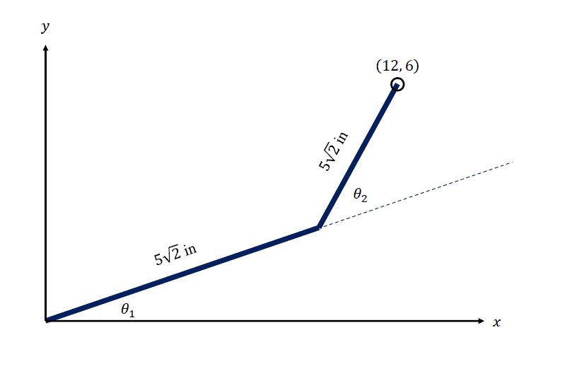
Figure 6. Two-link robot in Question 4.

Vectors

Vectors are essential in formulating engineering problems. They are defined geometrically as a line segment that starts at an initial point and ends with an arrow at a terminal point. With the initial point given by pi = (xi, yi) and the terminal point given by pt = (xt, yt) in a Cartesian grid, the vector can be written as

(13)

p = [\begin{matrix} x_{t} - x_{i} & y_{t} - y_{i} \end{matrix}] = [\begin{matrix} a & b \end{matrix}]

where the elements, a and b, of the vector are called the vector components. Vectors are defined by a magnitude and a direction, with the magnitude given by the length of the line and the direction indicating where the line is pointing. The magnitude of the vector p is given by

(14)

|p| = \sqrt{a^{2} + b^{2}}

and the direction can be calculated as

(15)

0 = \tan^{-1} (\frac{b}{a})

Two vectors are equal if their magnitude and direction are the same.

Vector addition and multiplication by a scalar can be considered geometrically as follows. Consider a vector u and a vector v that are to be added together. Placing the initial point of one vector in the same location as the terminal point of the other, the resultant summed vector can be found by connecting the initial point of the first vector to the terminal point of the second. This geometric interpretation of vector addition is shown in Fig. 7. Note that vector addition is commutative since the magnitude and direction of the resultant vector doesn’t depend on the order in which we add the vectors together.

$Geometric view of vector addition$

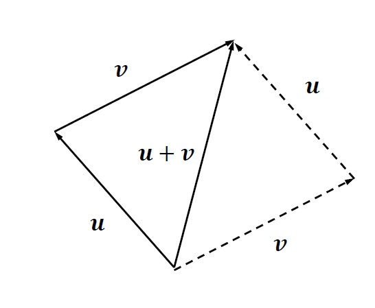
Figure 7. Geometric view of vector addition

Algebraically, vector addition is accomplished by adding the components of the two vectors. With the vector $u = [\begin{matrix} u_{1} & u_{2} \end{matrix}]$ and the vector $v = [\begin{matrix} v_{1} & v_{2} \end{matrix}]$ , the resultant vector from addition is given by

(16)

u + v = [\begin{matrix} u_{1} + v_{1} & u_{2} + v_{2} \end{matrix}]

Subtracting vectors is accomplished geometrically by simply switching the direction of the vector being subtracted and then performing a vector addition. This process is shown in Fig. 8 geometrically and is performed algebraically by subtracting the vector components from one another. Thus, subtracting the vector v from u gives

(17)

u + v = [\begin{matrix} u_{1} - v_{1} & u_{2} - v_{2} \end{matrix}]

$Geometric view of vector subtraction$

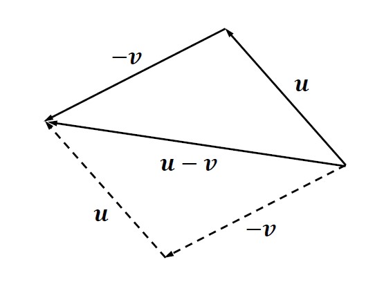
Figure 8. Geometric view of vector subtraction.

Scalar multiplication of a vector by a scalar is represented geometrically as simply scaling the magnitude of the vector without changing its direction. Geometrically, this is shown in Fig. 9 with a constant scalar γ applied to the vector. Algebraically, the scaling occurs by multiplying each component of the vector by the scalar value. In the case where the scalar value is given by γ, this process is given by

(18)

γ u = γ [\begin{matrix} a & b \end{matrix}] = [\begin{matrix} γa & γb \end{matrix}]

Equation (13) showed one way to represent vectors. Another common representation for vectors utilizes a unit vector notation. Unit vectors are vectors that have unit magnitude, meaning a magnitude of one. Any vector can be turned into a unit vector by dividing its components by the magnitude of the vector. Writing Eq. (13) in terms of the Cartesian unit vectors, i and j, we have

(19)

p = a i + b j

$Geometric view of vector scaling$

Figure 9. Geometric view of vector scaling.

Addition and subtraction of vectors in this form follows the same process as given in Eqs. (16) and (17). Having covered vector addition, subtraction, and scalar multiplication, we may wonder if there is an analog for multiplying vectors. Indeed, there are two ways in which to multiply vectors. Here, we will only consider the multiplication of vectors that results in a scalar product. This type of vector multiplication is called the dot product or scalar product. Geometrically, the dot product can be calculated using the magnitudes of the of the two vectors and the angle θ made between them. This is given by

(20)

u v = |u| |v| cos 0

Algebraically, so long as we know the components of the vectors, we can calculate the dot product as

(21)

u v = u_{1} v_{1} + u_{2} v_{2}

Question 5. You are pushing a lawn mower using 20 lbs. of force at an angle of 30° with the horizontal. What is the horizontal component, F_x, and the vertical component, F_y, of the force? See Fig. 10.

$Force on a lawn mower in Question 5$

Figure 10. Force on a lawn mower in Question 5.